Reading Notes of Learning Bayesian Networks(Neapolitan)
Bayesian networks looks like a game of conditional independence and dependence
Basics
A few quick review of basic probability theory
marginal probability: The summed probability of a joint probability $$P(A|B) = \sum_{C}P(A,C|B)$$
Law of total probability: $$P(A|C,D,E) = \sum_{B}P(A|B,C,D,E)P(B|C,D,E)$$ , which is nothing more than weighted average of the conditional probability of $A$ given $B$ and the marginal probability of $B$. The simplest form is $$P(A|B) = \sum_{C}P(A|B,C)P(C|B)$$ This is different from marginal probability above.
$\perp$ notation for independence: $$A \perp B|C$$ can be used to denote that $A$ and $B$ are independent given $C$. This is equivalent to $P(A,B|C) = P(A|C)P(B|C)$. This actually is more than handy because it does have a geometric interpretation of conditional independence. Check figure below.
Independence does not imply conditional independence: $$A \perp B \nRightarrow A \perp B|C$$ A counter-example is given in the figure below. And it seems that in our figure, which is a circle on 2D, we can not find an example that independence implies conditional independence unless we go to 3D or higher dimension.
How to know if two random variables are independent ? There seem to be two ways to know if two random variables $X$ and $Y$ are independent:
- For all possible values of $X$ and $Y$, check if the joint probability of $X$ and $Y$ is equal to the product of the marginal probability of $X$ and $Y$. That is, $P(X,Y) = P(X)P(Y)$, $O(n*m)$ time complexity
- Check if the conditional probability of $X$ given $Y$ is equal to the marginal probability of $X$. That is, $P(X|Y) = P(X)$, also $O(n*m)$ time complexity
Depending on we are given the joint or conditional probability, we can choose the corresponding method to check if two random variables are independent.
- Check conditional independence
Now let’s check if $X$ and $Y$ are independent given $Z_1, Z_2, …, Z_n$. By definition, $X$ and $Y$ are independent given $Z_1, Z_2, …, Z_n$ if and only if $P(X,Y|Z_1, Z_2, …, Z_n) = P(X|Z_1, Z_2, …, Z_n)P(Y|Z_1, Z_2, …, Z_n), \forall X, Y, Z_1, Z_2, …, Z_n$. This is a natural extension of the definition of independence between two random variables above. But the computational complexity is $O(m^n)$, which is intolerable. So there is no efficient way to check if two random variables are independent given a set of other random variables in general.
- Dependency is not transitive
Proposition 1: Depedency relationship between random variables are not transitive, i.e. if $X$ and $Y$ are dependent, and $Y$ and $Z$ are dependent, it does not imply $X$ and $Z$ are dependent. Below is an example, and it can be easily extend to case more than 3 random variables, as long as we have orthogonal dependency relationship between the head and tail of the chain.

Figure 1. Dependency Not Transitive
- Bayesian Inference
Just a quick review of Bayesian Inference.
It tells us how to get $P(X|Y)$ from $P(Y|X)$.
- conditional expectation
Conditional expectation has been a bit confusing to me at the beginning and the reason I think it’s because of the confusing notation.
$$E(X|Y) = E_{X|Y}[X] = \sum_{x}xP(X=x|Y)$$
$$E(X|Y,Z) = E_{X|Y,Z}[X] = \sum_{x}xP(X=x|Y,Z)$$
$$E[E(X|Y,Z)|Y] = E_{Z|Y}[E_{X|Y,Z}[X]] = E_{X|Y}[X] = E(X|Y)$$, known as law of iterated expectations or tower property
Chapter 1: Introduction to Bayesian Networks
Three definition of probability
This is the first interesting thing I learned from this book. The author introduced three definitions of probability:
- probability based on principal of indifference: For example in a coin flip, the probability of head is 0.5 because the two outcomes are symmetric and we just assign equal probability to them.
- probability based on frequentist: For event like throwing a thumbtack, we can not apply principal of indifference because the outcomes (head or tail) are not symmetric and are complicated. So we can only rely on the frequentist definition of probability, which is the ratio of the number of times the event occurs to the total number of trials.
- probability based on subjective: For example, when there is match between Brazil and Argentina in world cup, some people may think Brazil has probability of 0.6 to win, while others may think it is 0.7. Here the probability is clearly not based on the principal of indifference and also not based on frequentist because we can not repeat the match in the same(similar) condition many times. So the probability is a pure subjective estimation. This is still ok because the probability theory per se does not make any assumption on the nature of the probability but just the few axioms. Even though the probability is subjective, very far from reality, it is still a valid probability and we can apply all the probability theory ( including Bayesian Networks) to it.
Graph Description of Random Variables
The basic idea of Bayesian Networks is to use a graph to describe the relationship between random variables.
The graph $G$ needs to be carefully designed so that it is aligned with our interested probability distribution $P$.
The graph $G$ encodes conditional dependence and independence as edges and non-edges.
The graph itself can be seen as a compact representation of the joint probability distribution $P$.
There are at least two interesting questions to ask:
- Given a joint probability distribution $P$, how to find a graph $G$ that is consistent with $P$?
- Given a graph $G$, how to find a joint probability distribution $P$ that is consistent with $G$?
The first question is the learning problem, while the second question is the inference problem.
The inference problem is easy because we can simply use the chain rule to get the joint probability distribution $P$ from the graph $G$.
The learning problem is hard because we need to accomplish at least two hard tasks:
- make sure the structure of the graph $G$ is consistent with the joint probability distribution $P$, i.e. dependency and independency between random variables
- compute the conditional probability distribution of dependent variables in the graph $G$.
The 1st task is hard and I don’t know yet how to do it, I guess the following chapters will tell me. The 2nd task is easy because we just need to marginalize to get the conditional probability distribution we want.
No One-to-One Correspondence between Graph and Probability Distribution
The author gave a simple motivating example and it seems to show that there is no one-to-one correspondence between graph and probability distribution.
More concretely, multiple graphs $G_1, G_2, …, G_n$ can represent the same probability distribution $P$. (But the reverse is not true, i.e. one graph can only represent one probability distribution)
Below is the example:
Here we list the joint probability distribution of the random variables $C, S, V$:
- C stands for the color,
- S stands for the shape,
- V stands for the volume.
| C | S | V | P(C, S, V) |
|---|---|---|---|
| Black | Circle | 1 | 1/13 |
| Black | Circle | 2 | 2/13 |
| Black | Square | 1 | 2/13 |
| Black | Square | 2 | 4/13 |
| White | Circle | 1 | 1/13 |
| White | Circle | 2 | 1/13 |
| White | Square | 1 | 1/13 |
| White | Square | 2 | 1/13 |
First, it is suprising to me that given this joint probability distribution, it’s definitely not trivial to know the conditional independence of $C, S, V$ by just looking at the table without doing any calculation.
And it seems there is indeed no more efficient way to check the conditional independence without doing the calculation above, which is $O(m^n)$.
The conclusions are:
- V and C are dependent
- black favors 2, white favors 1
- V and S are dependent
- circle favors 1, square favors 2
- C and S are dependent
- black favors square, white favors circle
Conditional Independence:
- $I(V, C|S)$
- $P(V|S) = P(V|C, S)$
- Under Square, black favors 2, white favors 1
- Under Circle, black favors 2, white favors 1
- $P(V|S) = P(V|C, S)$
- $I(V, S|C)$
- $P(V|C) = P(V|S, C)$
- Under Black, circle doesn’t provide any information about value
- Under White, circle doesn’t provide any information about value
- $P(V|C) = P(V|S, C)$
- $I(C, S|V)$
- $P(C|V) = P(C|S, V)$
- Under 1, circle favors white, square favors black
- Under 2, circle favors white, square favors black
- $P(C|V) = P(C|S, V)$
So there is one conditional independence, i.e. $I(V, C|S)$, and the rest are dependent.
Graph
Given the three random variables $C, S, V$, the book gave 4 possible graphs struture and only 3 of them are valid.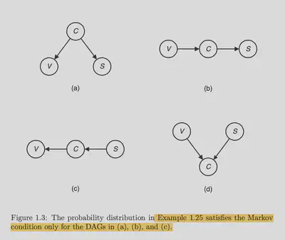
It is not hard to see that given 3 random variables, there are:
- $V$ shape graph: 3 possible graphs
- The parent two nodes $A$ and $B$ have to be independent. In other words, the $V$ shape graph has the property that $P(A=a, B=b) = \sum_{c}P(A=a, B=b, C=c) = \sum_{c}P(A=a)P(B=b)P(C=c|A=a, B=b) = P(A=a)P(B=b)$. So this structure already implies the independence between $A$ and $B$.
- But $A$ and $B$ also must be dependent given the child $C$, unless the graph is degenerated, i.e. $B$ and $C$ or $A$ and $C$ are indepdent. Check the example above about non-transitive dependency.
- $A$ shape graph: 3 possible graphs
- No specific constraint, the two child nodes can be dependent or independent.
- The two children can be independent or dependent given the parent ( see the transive dependency example above)
- $I$ shape graph: 6 possible graphs
- The $I$ shape graph has a strong constraint of conditional independence.
$V$ shape graph is the d graph in above figure, $A$ shape graph is the a graph in above figure, and $I$ shape graph is the b, c graphs in above figure.
The good thing about categorizing the graph structure into three types is that any big graph is just a combination of these three types of graphs.
So there are 12 possible graphs in total, below I list all of them:
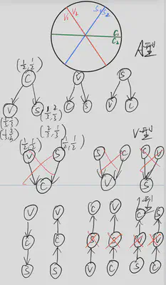
And because our joint probability distribution has dependency relationship between $C, S, V$, we can rule out the $V$ shape graph, and we are left with 9 possible graphs. We can further rule out $\frac{4}{6}$ of the $I$ shape graph because they have conditional independence between $C, S, V$.
So we are left with 5 possible graphs and they are all valid.
Below is a graph that contains 5 random variables and we can see that it can be decomposed into 1 $V$ shape graph,1 $A$ shape graph and 3 $I$ shape graphs.
D-separation
D-separation means dependency separation.
It basically answers the question: Is $X$ and $Y$ independent given $Z_1, Z_2, …, Z_n$?
Here is a great tutorial to learn the “algorithm” of D-separation: D-separation
Saibo Geng
PhD student in EPFL
My research interest is improving LLM’s performance through decoding methods.